import subprocess
import sys

COLAB = "google.colab" in sys.modules


def _install(package):
    if COLAB:
        ans = input(f"Install { package }? [y/n]:")
        if ans.lower() in ["y", "yes"]:
            subprocess.check_call(
                [sys.executable, "-m", "pip", "install", "--quiet", package]
            )
            print(f"{ package } installed!")


def _colab_install_missing_deps(deps):
    import importlib

    for dep in deps:
        if importlib.util.find_spec(dep) is None:
            if dep == "iris":
                dep = "scitools-iris"
            _install(dep)


deps = ["cf_xarray", "erddapy", "ioos_qc"]
_colab_install_missing_deps(deps)

IOOS QARTOD software (ioos_qc)¶

Created: 2020-02-14

Updated: 2022-05-23

This post will demonstrate how to run ioos_qc on a time-series dataset. ioos_qc implements the Quality Assurance / Quality Control of Real Time Oceanographic Data (QARTOD).

We will be using the water level data from a fixed station in Kotzebue, AK.

Below we create a simple Quality Assurance/Quality Control (QA/QC) configuration that will be used as input for ioos_qc. All the interval values are in the same units as the data.

For more information on the tests and recommended values for QA/QC check the documentation of each test and its inputs: https://ioos.github.io/ioos_qc/api/ioos_qc.html#module-ioos_qc.qartod

qc_config = {
    "qartod": {
        "gross_range_test": {"fail_span": [-10, 10], "suspect_span": [-2, 3]},
        "flat_line_test": {
            "tolerance": 0.001,
            "suspect_threshold": 10800,
            "fail_threshold": 21600,
        },
        "spike_test": {
            "suspect_threshold": 0.8,
            "fail_threshold": 3,
        },
    }
}

Now we are ready to load the data, run tests and plot results!

We will get the data from the AOOS ERDDAP server.

import cf_xarray

print(cf_xarray.__version__)
from erddapy import ERDDAP

e = ERDDAP(server="https://erddap.aoos.org/erddap/", protocol="tabledap")
e.dataset_id = "kotzebue-alaska-water-level"
e.constraints = {
    "time>=": "2018-09-05T21:00:00Z",
    "time<=": "2019-07-10T19:00:00Z",
}

data = e.to_xarray()

data.cf

0.8.4

Discrete Sampling Geometry:
            CF Roles:   timeseries_id: ['station']

Coordinates:
             CF Axes:   X: ['longitude']
                        Y: ['latitude']
                        T: ['time']
                        Z: n/a

      CF Coordinates:   longitude: ['longitude']
                        latitude: ['latitude']
                        time: ['time']
                        vertical: n/a

       Cell Measures:   area, volume: n/a

      Standard Names:   latitude: ['latitude']
                        longitude: ['longitude']
                        time: ['time']

              Bounds:   n/a

       Grid Mappings:   n/a

Data Variables:
       Cell Measures:   area, volume: n/a

      Standard Names:   aggregate_quality_flag: ['sea_surface_height_above_sea_level_geoid_mhhw_qc_agg']
                        altitude: ['z']
                        sea_surface_height_above_sea_level: ['sea_surface_height_above_sea_level_geoid_mhhw']
                        sea_surface_height_above_sea_level quality_flag: ['sea_surface_height_above_sea_level_geoid_mhhw_qc_tests']

              Bounds:   n/a

       Grid Mappings:   n/a

from ioos_qc.config import QcConfig

qc = QcConfig(qc_config)

# The result is always a list but we only want the first, one and only in this case, variable.
variable_name = data.cf.standard_names["sea_surface_height_above_sea_level"][0]

qc_results = qc.run(
    inp=data[variable_name],
    tinp=data.cf["T"].to_numpy(),
)

qc_results

defaultdict(collections.OrderedDict,
            {'qartod': OrderedDict([('gross_range_test',
                           array([1, 1, 1, ..., 1, 1, 1], dtype=uint8)),
                          ('flat_line_test',
                           array([1, 1, 1, ..., 1, 1, 1], dtype=uint8)),
                          ('spike_test',
                           array([2, 1, 1, ..., 1, 1, 2], dtype=uint8))])})

The results are returned in a dictionary format, similar to the input configuration, with a mask for each test. While the mask is a masked array it should not be applied as such. The results range from 1 to 4 meaning:

data passed the QA/QC
did not run on this data point
flag as suspect
flag as failed

Now we can write a plotting function that will read these results and flag the data.

import matplotlib.pyplot as plt
import numpy as np


def plot_results(data, variable_name, results, title, test_name):
    time = data.cf["time"]
    obs = data[variable_name]
    qc_test = results["qartod"][test_name]

    qc_pass = np.ma.masked_where(qc_test != 1, obs)
    qc_suspect = np.ma.masked_where(qc_test != 3, obs)
    qc_fail = np.ma.masked_where(qc_test != 4, obs)
    qc_notrun = np.ma.masked_where(qc_test != 2, obs)

    fig, ax = plt.subplots(figsize=(15, 3.75))
    fig.set_title = f"{test_name}: {title}"

    ax.set_xlabel("Time")
    ax.set_ylabel("Observation Value")

    kw = {"marker": "o", "linestyle": "none"}
    ax.plot(time, obs, label="obs", color="#A6CEE3")
    ax.plot(
        time, qc_notrun, markersize=2, label="qc not run", color="gray", alpha=0.2, **kw
    )
    ax.plot(
        time, qc_pass, markersize=4, label="qc pass", color="green", alpha=0.5, **kw
    )
    ax.plot(
        time,
        qc_suspect,
        markersize=4,
        label="qc suspect",
        color="orange",
        alpha=0.7,
        **kw,
    )
    ax.plot(time, qc_fail, markersize=6, label="qc fail", color="red", alpha=1.0, **kw)
    ax.grid(True)


title = "Water Level [MHHW] [m] : Kotzebue, AK"

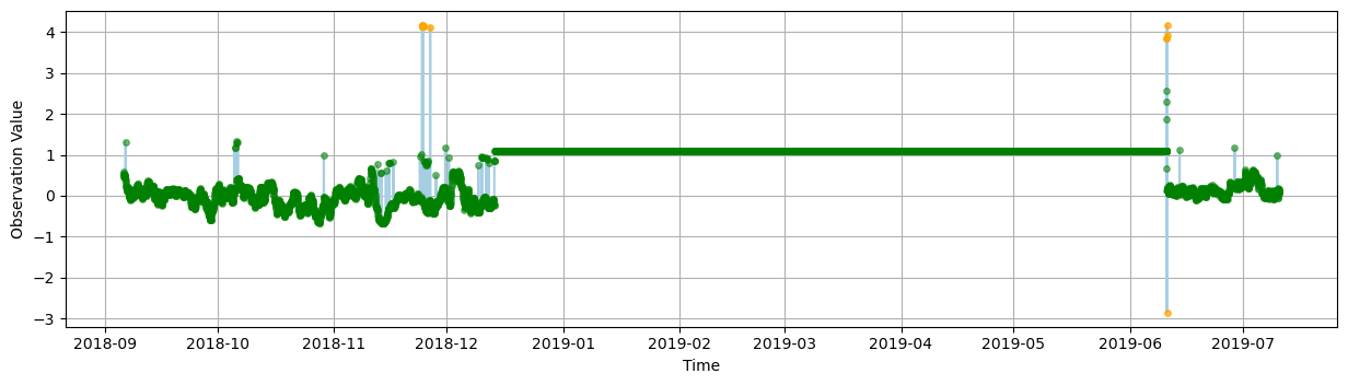
The gross range test test should fail data outside the $\\pm$ 10 range and suspect data below -2, and greater than 3. As one can easily see all the major spikes are flagged as expected.

plot_results(
    data,
    variable_name,
    qc_results,
    title,
    "gross_range_test",
)

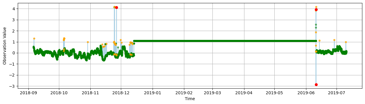
An actual spike test, based on a data increase threshold, flags similar spikes to the gross range test but also indetifies other suspect unusual increases in the series.

plot_results(
    data,
    variable_name,
    qc_results,
    title,
    "spike_test",
)

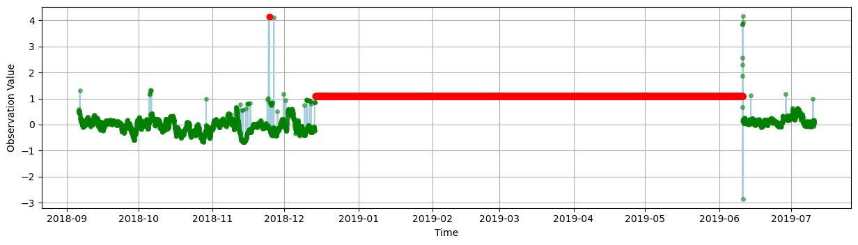
The flat line test identifies issues with the data where values are “stuck.”

ioos_qc succefully identified a huge portion of the data where that happens and flagged a smaller one as suspect. (Zoom in the red point to the left to see this one.)

plot_results(
    data,
    variable_name,
    qc_results,
    title,
    "flat_line_test",
)

This notebook was adapted from Jessica Austin and Kyle Wilcox’s original ioos_qc examples. Please see the ioos_qc documentation for more examples.