Created: 2024-05-16
Updated: 2024-07-02
This notebook walks through downloading a netCDF file from NCEI. The file follows a specific specification for ATN satellite trajectory observations as documented here. More information about the ATN netCDF specification can be found at https://
Since most of the examples in the IOOS Code Lab are in the python programming language, we wanted to show an example of working with a netCDF file in the R programming language to be inclusive of those users.
For more information on the tidync package, see this R blog: https://
Data used in this notebook are available from NCEI at the following link https://
library(tidync)
library(obistools)
library(ncdf4)
library(tidyverse)
library(lubridate)
library(maps)
library(mapdata)
The legacy packages maptools, rgdal, and rgeos, underpinning the sp package,
which was just loaded, will retire in October 2023.
Please refer to R-spatial evolution reports for details, especially
https://r-spatial.org/r/2023/05/15/evolution4.html.
It may be desirable to make the sf package available;
package maintainers should consider adding sf to Suggests:.
The sp package is now running under evolution status 2
(status 2 uses the sf package in place of rgdal)
-- Attaching packages ----------------------------------------------------------------------------------------------------------------------------------------------------------------------------------------------- tidyverse 1.3.2 --
v ggplot2 3.4.2 v purrr 1.0.1
v tibble 3.2.1 v dplyr 1.1.1
v tidyr 1.3.0 v stringr 1.5.0
v readr 2.1.4 v forcats 1.0.0
-- Conflicts -------------------------------------------------------------------------------------------------------------------------------------------------------------------------------------------------- tidyverse_conflicts() --
x dplyr::filter() masks stats::filter()
x dplyr::lag() masks stats::lag()
Attaching package: 'lubridate'
The following objects are masked from 'package:base':
date, intersect, setdiff, union
Attaching package: 'maps'
The following object is masked from 'package:purrr':
map
Download the netCDF file from the NCEI Archive
url = 'https://www.ncei.noaa.gov/data/oceans/archive/arc0217/0282699/1.1/data/0-data/atn_45866_great-white-shark_trajectory_20090923-20091123.nc'

fname = basename(url)

download.file(url, fname, mode = "wb")
Collect all the metadata from the netCDF file.
This gathers not only the global attributes, but the variable level attributes as well. As you can see in the variable column the term NC_GLOBAL refers to global attributes.
metadata <- ncmeta::nc_atts(fname)Example extracting attributes from netCDF
To give you an idea of what observations are in this file, we can print out the human readable summary and long_name attributes from all the variables.
metadata %>% dplyr::filter(name == "summary")metadata %>% dplyr::filter(name == "long_name")Store the data as a tibble in a variable
Collect the data dimensioned by time from the netCDF file as a tibble. Then, print the first few rows.
atn <- tidync(fname)

atn_tbl <- atn %>% hyper_tibble(force=TRUE)

head(atn_tbl, n=4)Dealing with time
Notice the data in the time column aren’t formatted as times. We need to read the metadata associated with the time variable to understand what the units are. Below, we print a tibble of all the attributes from the time variable.
Notice the units attribute and it’s value of seconds since 1990-01-01 00:00:00Z. We need to use that information to convert the time variable to something useful that ggplot can handle.
time_attrs <- metadata %>% dplyr::filter(variable == "time")
time_attrsSo, we grab the value from the units attribute, split the string to collect the date information, and apply that to a time conversion function as.POSIXct.
tunit <- time_attrs %>% dplyr::filter(name == "units")
lunit <- str_split(tunit$value,' ')[[1]]
atn_tbl$time <- as.POSIXct(atn_tbl$time, origin=lunit[3], tz="GMT")

head(atn_tbl, n=2)Plotting the raw data
Now lets make some plots just to take a look at what data we’re working with. Here we make a plot of time vs longitude.
options(repr.plot.width = 20, repr.plot.height = 7)

# collect title from global attributes
title <- metadata %>% dplyr::filter(variable == "NC_GLOBAL") %>% dplyr::filter(name == "title")

# Map limits.
ylim <- c( min(atn_tbl$lat)-0.25, max(atn_tbl$lat)+0.25 )
xlim <- c( min(atn_tbl$lon)-0.25, max(atn_tbl$lon)+0.25 )

# Get outline data for map.
w <- map_data( 'worldHires', ylim = ylim, xlim = xlim )

z <- ggplot(atn_tbl, aes( x = lon, y = lat )) +
     geom_point( aes(color=location_class), size=2) +
     geom_line( color = 'grey' ) +
     scale_shape_manual( values = c(19, 1) )

z + geom_polygon(data = w, aes(x = long, y = lat, group = group), fill = 'grey80') +
    theme_bw() +
    coord_fixed(1.3, xlim = xlim, ylim = ylim) +
    labs(title = paste( strwrap(title$value, width = 150), collapse = "\n"))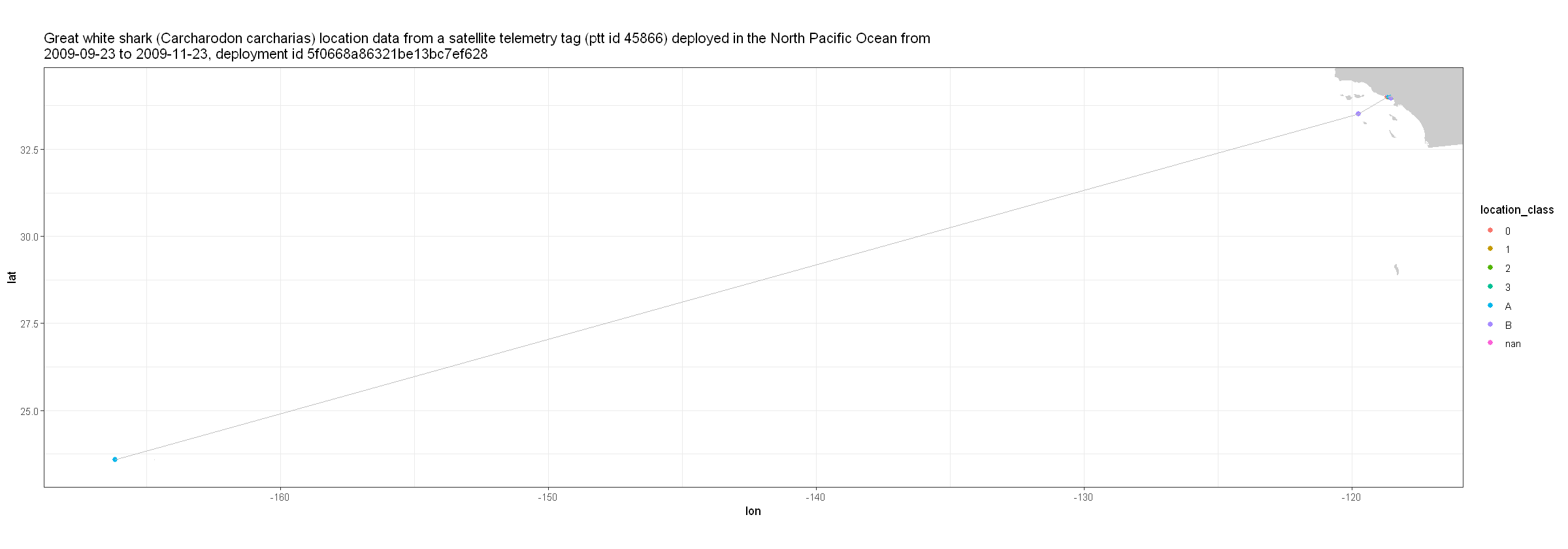
What do these location_class codes mean?
code_defs <- metadata %>% dplyr::filter(variable == "location_class") %>% dplyr::filter(name=="code_meanings" | name=="code_values")

str_split_fixed(code_defs$value,",",8)Review location uncertainty information and map to how many meters the uncertainty is.
From the table above, only nan, G, 3, 2, 1, and 0 are valid points with known undertainties.
atn_tbl_qc <- atn_tbl %>%
    filter(location_class %in% c('nan','G','3','2','1','0')) %>%
#     mutate(  # This returns NA for any other values than those defined below
#         coordinateUncertaintyInMeters = case_when(location_class == 'nan' ~ 0,
#                                                      location_class == 'G' ~ 200,
#                                                      location_class == '3' ~ 250,
#                                                      location_class == '2' ~ 500,
#                                                      location_class == '1' ~ 1500,
#                                                      location_class == '0' ~ 10000) # https://github.com/ioos/bio_data_guide/issues/145#issuecomment-1805739244
#           ) %>%
    arrange(time)

head(atn_tbl_qc)Making a map
Next, let’s make a map of the locations of this animal with the colors identifying the location classes described in the table above.
options(repr.plot.width = 10, repr.plot.height = 10)

# collect title from global attributes
title <- metadata %>% dplyr::filter(variable == "NC_GLOBAL") %>% dplyr::filter(name == "title")

# Map limits.
ylim <- c( min(atn_tbl_qc$lat)-0.15, max(atn_tbl_qc$lat)+0.15 )
xlim <- c( min(atn_tbl_qc$lon)-0.15, max(atn_tbl_qc$lon)+0.15 )

# Get outline data for map.
w <- map_data( 'worldHires', ylim = ylim, xlim = xlim )

z <- ggplot(atn_tbl_qc, aes( x = lon, y = lat )) +
     geom_point( aes(color = location_class, size = 2 )) +
     geom_line( color='grey' ) +
     scale_shape_manual( values = c(19, 1) )

z + geom_polygon(data = w, aes(x = long, y = lat, group = group), fill = 'grey80') +
    theme_bw() +
    coord_fixed(1.3, xlim = xlim, ylim = ylim) +
    labs(title = paste( strwrap(title$value, width = 150), collapse = "\n"))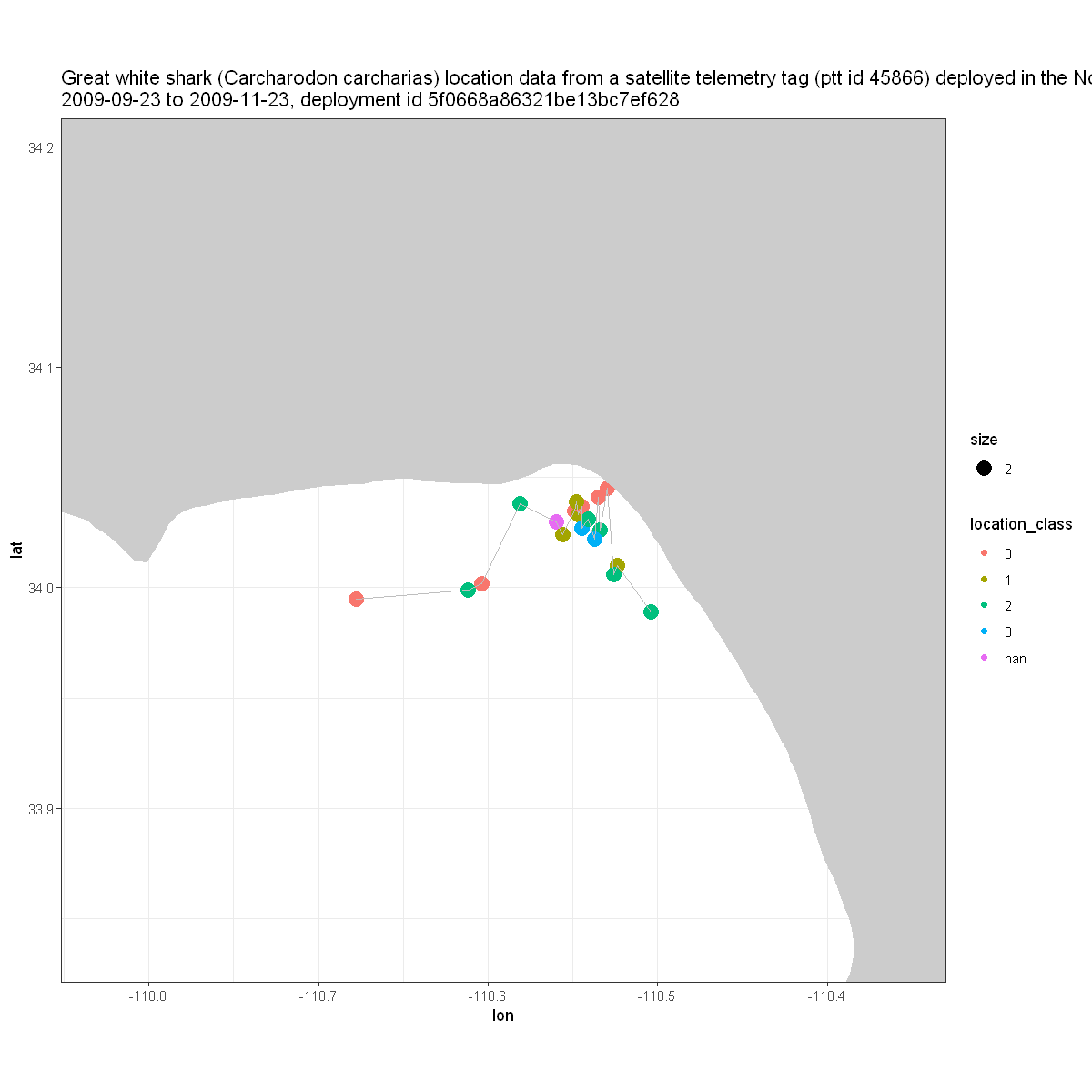
Interpolating MURSST to white shark tracks using ERDDAP
The MURSST product is a merged, multi-sensor L4 Foundation Sea Surface Temperature (SST) analysis product from Jet Propulsion Laboratory (JPL).
This daily, global, Multi-scale, Ultra-high Resolution (MUR) Sea Surface Temperature (SST) 1-km data set, Version 4.1, is produced at JPL under the NASA MEaSUREs program.
For details, see https://
We need to prepare the data to send to the server. As mentioned above the request will take a table with a header "time,latitude,longitude", then its values. Note that we rename the columns, then pick the subset to store as one long string to create the request.
time_lat_lon <- atn_tbl_qc %>%
    rename(
        latitude = lat,
        longitude = lon)

time_lat_lon <- format_csv(time_lat_lon[c('time','latitude','longitude')])
The cell below builds the request and download get it back as a data.frame.
response = "csv"
dataset_id = "jplMURSST41"
variable = "analysed_sst"
algorithm = "Nearest"
nearby = 216

url = paste0(
    "http://coastwatch.pfeg.noaa.gov/erddap/",
    "convert/interpolate.",response,
    "?TimeLatLonTable=",URLencode(time_lat_lon, reserved=TRUE),
    "&requestCSV=",dataset_id,
    "/",variable,
    "/",algorithm,
    "/",nearby
)

df <- read.csv(url)
Now let’s plot what the interpolated sea surface temperatures were for that animal at that location and time.
options(repr.plot.width = 10, repr.plot.height = 10)

# collect title from global attributes
title <- metadata %>% dplyr::filter(variable == "NC_GLOBAL") %>% dplyr::filter(name == "title")

# Map limits.
ylim <- c( min(df$latitude)-0.1, max(df$latitude)+0.1 )
xlim <- c( min(df$longitude)-0.1, max(df$longitude)+0.1 )

# Get outline data for map.
w <- map_data( 'worldHires', ylim = ylim, xlim = xlim )

z <- ggplot(df, aes( x = longitude, y = latitude )) +
     geom_point( aes(color = jplMURSST41_analysed_sst_Nearest_216, size=2)) +
     geom_line() +
     scale_shape_manual( values = c(22, 17) ) +
     scale_color_gradient(low="blue", high="red")

z + geom_polygon(data = w, aes(x = long, y = lat, group = group), fill = 'grey80') +
    theme_bw() +
    coord_fixed(1.3, xlim = xlim, ylim = ylim) +
    labs(title = paste( strwrap(title$value, width = 200), collapse = "\n"))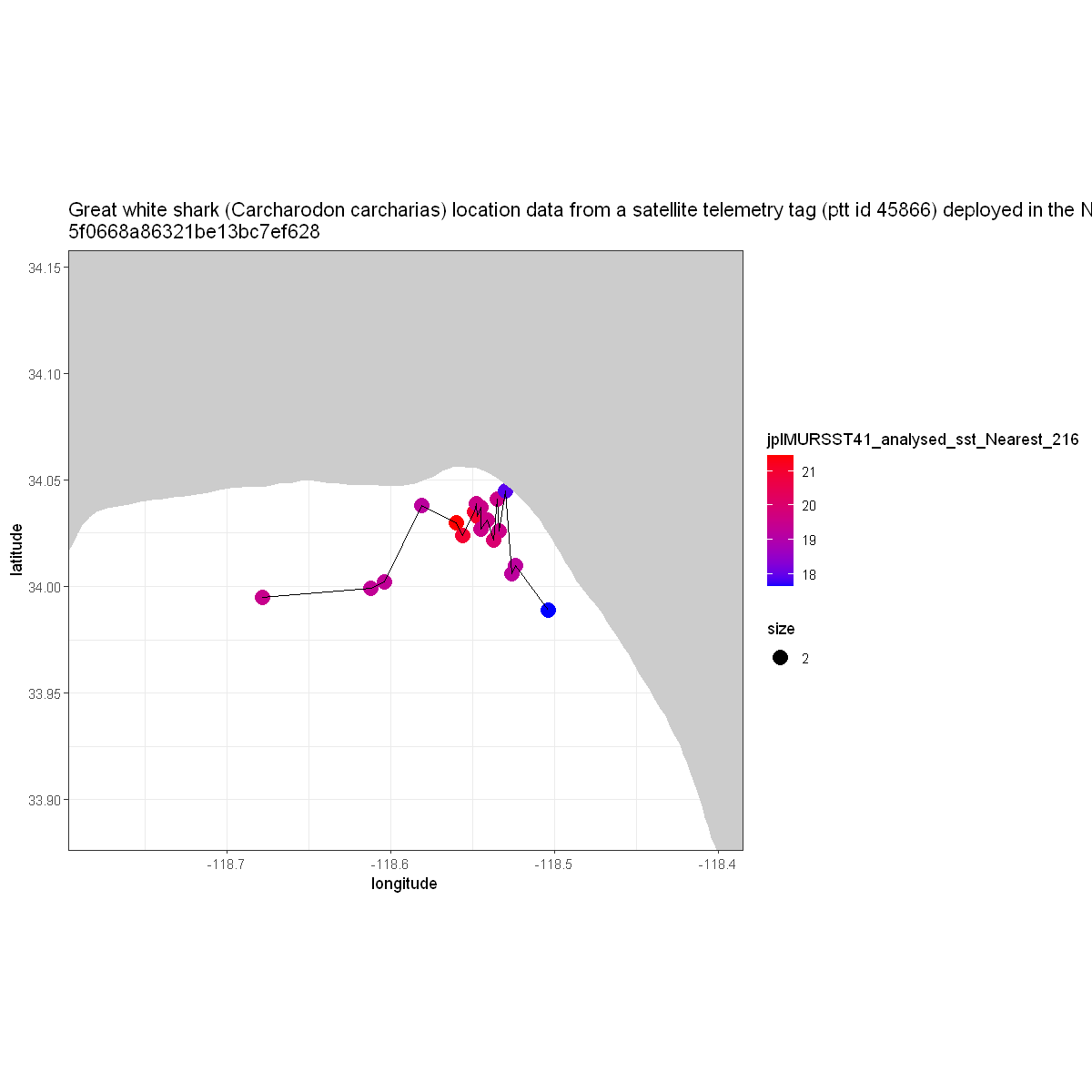
sessionInfo()R version 4.1.3 (2022-03-10)
Platform: x86_64-w64-mingw32/x64 (64-bit)
Running under: Windows 10 x64 (build 19045)
Matrix products: default
locale:
[1] LC_COLLATE=English_United States.1252
[2] LC_CTYPE=English_United States.1252
[3] LC_MONETARY=English_United States.1252
[4] LC_NUMERIC=C
[5] LC_TIME=English_United States.1252
attached base packages:
[1] stats graphics grDevices utils datasets methods base
other attached packages:
[1] mapdata_2.3.1 maps_3.4.1 lubridate_1.9.2 forcats_1.0.0
[5] stringr_1.5.0 dplyr_1.1.1 purrr_1.0.1 readr_2.1.4
[9] tidyr_1.3.0 tibble_3.2.1 ggplot2_3.4.2 tidyverse_1.3.2
[13] ncdf4_1.21 obistools_0.0.10 tidync_0.3.0
loaded via a namespace (and not attached):
[1] httr_1.4.6 bit64_4.0.5 vroom_1.6.1
[4] jsonlite_1.8.4 modelr_0.1.11 sp_2.0-0
[7] googlesheets4_1.1.0 cellranger_1.1.0 pillar_1.9.0
[10] backports_1.4.1 lattice_0.20-45 glue_1.6.2
[13] uuid_1.1-0 digest_0.6.31 rvest_1.0.3
[16] colorspace_2.1-0 htmltools_0.5.5 pkgconfig_2.0.3
[19] broom_1.0.4 haven_2.5.2 scales_1.2.1
[22] tzdb_0.3.0 timechange_0.2.0 googledrive_2.1.0
[25] farver_2.1.1 generics_0.1.3 withr_2.5.0
[28] repr_1.1.6 cli_3.6.0 readxl_1.4.2
[31] magrittr_2.0.3 crayon_1.5.2 evaluate_0.20
[34] data.tree_1.0.0 fs_1.6.1 fansi_1.0.4
[37] xml2_1.3.3 tools_4.1.3 hms_1.1.3
[40] geosphere_1.5-18 gargle_1.4.0 lifecycle_1.0.3
[43] reprex_2.0.2 munsell_0.5.0 compiler_4.1.3
[46] RNetCDF_2.6-2 rlang_1.1.0 grid_4.1.3
[49] pbdZMQ_0.3-9 IRkernel_1.3.2 rappdirs_0.3.3
[52] htmlwidgets_1.6.2 crosstalk_1.2.0 labeling_0.4.2
[55] base64enc_0.1-3 rmarkdown_2.20 gtable_0.3.3
[58] DBI_1.1.3 R6_2.5.1 ncmeta_0.3.5
[61] knitr_1.42 bit_4.0.5 fastmap_1.1.1
[64] rgeos_0.6-2 utf8_1.2.3 stringi_1.7.12
[67] parallel_4.1.3 IRdisplay_1.1 Rcpp_1.0.10
[70] vctrs_0.6.1 leaflet_2.1.2 dbplyr_2.3.2
[73] tidyselect_1.2.0 xfun_0.37