import subprocess
import sys

COLAB = "google.colab" in sys.modules


def _install(package):
    if COLAB:
        ans = input(f"Install { package }? [y/n]:")
        if ans.lower() in ["y", "yes"]:
            subprocess.check_call(
                [sys.executable, "-m", "pip", "install", "--quiet", package]
            )
            print(f"{ package } installed!")


def _colab_install_missing_deps(deps):
    import importlib

    for dep in deps:
        if importlib.util.find_spec(dep) is None:
            if dep == "iris":
                dep = "scitools-iris"
            _install(dep)


deps = ["cartopy"]
_colab_install_missing_deps(deps)

Calling R libraries from Python¶

Created: 2017-11-30

In this example we will explore the Coral Reef Evaluation and Monitoring Project (CREMP) data available in the Gulf of Mexico Coastal Ocean Observing System (GCOOS) ERDDAP server.

To access the server we will use the rerddap library and export the data to Python for easier plotting.

The first step is to load the rpy2 extension that will allow us to use the R libraries.

%load_ext rpy2.ipython

The first line below has a %%R to make it an R cell. The code below specify the GCOOS server and fetches the data information for the fk_CREMP_yearly_revisited_DATA_v3_1996 dataset.

For more information on rerddap please see https://docs.ropensci.org/rerddap/.

%%R

library('rerddap')

url <- 'https://gcoos4.tamu.edu/erddap'
data_info <- rerddap::info('fk_CREMP_yearly_revisited_DATA_v3_1996', url=url)

data_info

<ERDDAP info> fk_CREMP_yearly_revisited_DATA_v3_1996 
 Base URL: https://gcoos4.tamu.edu/erddap 
 Dataset Type: tabledap 
 Variables:  
     acceptedNameAuthorship: 
     acceptedNameUsage: 
     acceptedNameUsageID: 
     averageNumberOfPoints: 
         Range: 407, 900 
         Units: count 
     basisOfRecord: 
     bottomType: 
     class: 
     country: 
     crs: 
     datasetID: 
     datasetName: 
     depth: 
         Range: 3.0, 54.0 
         Units: m 
     eventDate: 
         Range: 1996, 1996 
         Units: unknown 
     eventID: 
     family: 
     firstYear: 
         Range: 1996, 1996 
         Units: unknown 
     genus: 
     geodeticDatum: 
     habitat: 
     habitatID: 
     kingdom: 
     language: 
     latitude: 
         Range: 24.4517, 25.2953 
         Units: degrees_north 
     license: 
     locality: 
     longitude: 
         Range: -81.9195, -80.2087 
         Units: degrees_east 
     maximumDepthInMeters: 
         Range: 3.0, 54.0 
         Units: m 
     minimumDepthInMeters: 
         Range: 3.0, 54.0 
         Units: m 
     Observations: 
         Range: 0, 11839 
     occurrenceID: 
     occurrenceStatus: 
     order: 
     organismQuantity: 
         Range: 0.0, 0.9475 
         Units: 0.01percent 
     organismQuantityType: 
     ownerInstitutionCode: 
     phylum: 
     recordedBy: 
     samplingEffort: 
     samplingProtocol: 
     scientificName: 
     scientificNameAuthorship: 
     scientificNameID: 
     siteCode: 
     siteID: 
         Range: 10, 81 
         Units: unknown 
     siteName: 
     specificEpithet: 
     stateProvince: 
     stationNumber: 
         Range: 101, 814 
         Units: unknown 
     subRegionID: 
     taxonomicStatus: 
     taxonRank: 
     time: 
         Range: 8.283168E8, 8.283168E8 
         Units: seconds since 1970-01-01T00:00:00Z 
     transectLengthInMeters: 
         Range: 19.0, 26.0 
         Units: m 
     type: 
     vernacularName: 
     waterBody:

By inspecting the information above we can find the variables available in the dataset and use the tabledap function to download them.

Note that the %%R -o rdf will export the rdf variable back to the Python workspace.

%%R -o df

fields <- c(
    'depth',
    'longitude',
    'latitude',
    'organismQuantity',
    'genus',
    'habitat'
)

df <- tabledap(
    data_info,
    fields=fields,
    url=url
)

R[write to console]: info() output passed to x; setting base url to: https://gcoos4.tamu.edu/erddap

Now we need to export the R DataFrame to a pandas objects and ensure that all numeric types are numbers and not strings.

import pandas as pd

cols = ["longitude", "latitude", "depth", "organismQuantity"]
df[cols] = df[cols].apply(pd.to_numeric)

df.head()

We can navigate to ERDDAP’s info page to find the variables description. Let’s check what is organismQuantity:

The is value of the derived information product, such as the numerical value for biomass. This term does not include units. Mean number of observed fish per species for 5 Minutes

We can see that organismQuantity has a lot of zero values, let’s remove that first to plot the data positions only where something was found.

# Filter invalid values (-999).

cremp_1996 = df.loc[df["organismQuantity"] >= 0]
cremp_1996["genus"] = cremp_1996["genus"].str.strip()
cremp_1996.head()

What is the most common genus of Coral observed?

avg = cremp_1996.drop("habitat", axis=1).groupby("genus").mean()

avg

rerddap’s info request does not have enough metadata about the variables to explain the blank, and most abundant, genus. Checking the sever did not help figure that out. We’ll remove that for now to deal with only those that are identified.

cremp_1996 = cremp_1996.loc[cremp_1996["genus"] != ""]

There are also many genus with zero biomass count. In this example we’ll choose to do a biased analysis of occurrence and eliminate those where nothing was observed.

# Filter zero values (nothing was observed).

cremp_1996 = cremp_1996.loc[cremp_1996["organismQuantity"] > 0]

Now we can check the quantificationValue average by genus.

%matplotlib inline

avg = (
    cremp_1996.drop("habitat", axis=1).groupby("genus").mean()
)  # re-compute the "biased" average.
ax = avg["organismQuantity"].plot(kind="bar")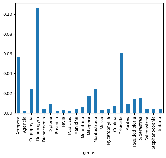

and habitat.

ax = (
    cremp_1996.drop("genus", axis=1)
    .groupby("habitat")
    .mean()["organismQuantity"]
    .plot(kind="bar")
)

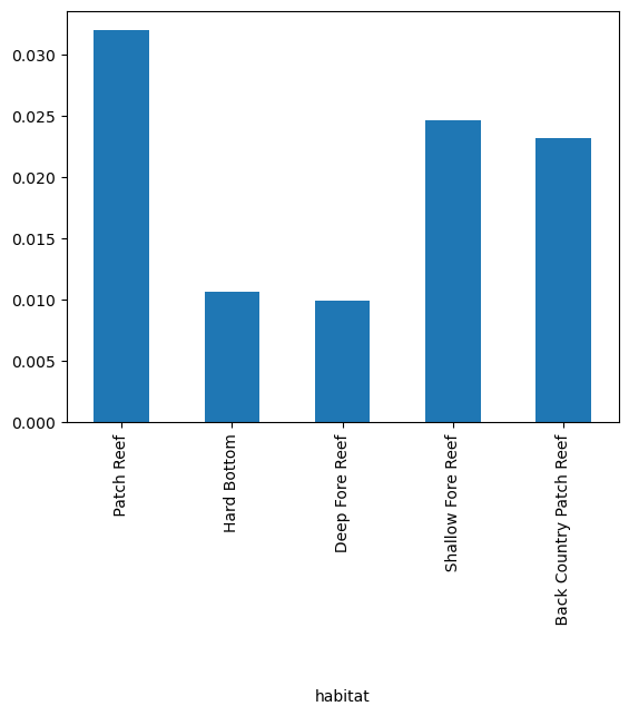
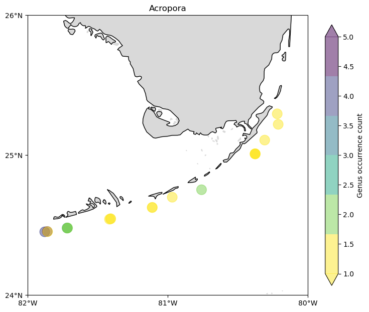
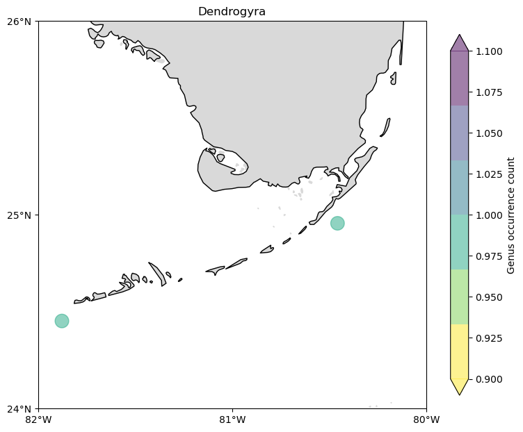
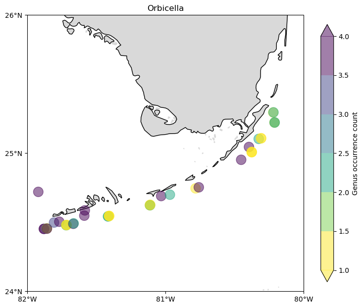
It seems the most of the biomass was found around the Dendrogyra genus in Patch Reef habitats. But where are those Coral Reefs? How is the distribution of top three species with more biomass around them? With a pandas DataFrame it is easy to group the data by location and count the genus occurrence based on it.

import cartopy.crs as ccrs
import cartopy.feature as cfeature
import matplotlib.pyplot as plt
import numpy as np
from cartopy.mpl.ticker import LatitudeFormatter, LongitudeFormatter


def make_plot():
    bbox = [-82, -80, 24, 26]
    projection = ccrs.PlateCarree()

    fig, ax = plt.subplots(figsize=(9, 9), subplot_kw=dict(projection=projection))

    ax.set_extent(bbox)

    land = cfeature.NaturalEarthFeature(
        "physical", "land", "10m", edgecolor="face", facecolor=[0.85] * 3
    )

    ax.add_feature(land, zorder=0)
    ax.coastlines("10m", zorder=1)

    ax.set_xticks(np.linspace(bbox[0], bbox[1], 3), crs=projection)
    ax.set_yticks(np.linspace(bbox[2], bbox[3], 3), crs=projection)
    lon_formatter = LongitudeFormatter(zero_direction_label=True)
    lat_formatter = LatitudeFormatter()
    ax.xaxis.set_major_formatter(lon_formatter)
    ax.yaxis.set_major_formatter(lat_formatter)
    return fig, ax

count = (
    cremp_1996.loc[cremp_1996["genus"] == "Acropora"]
    .groupby(["longitude", "latitude"])
    .count()
    .reset_index()
)


fig, ax = make_plot()
c = ax.scatter(
    count["longitude"],
    count["latitude"],
    s=200,
    c=count["genus"],
    alpha=0.5,
    cmap=plt.cm.get_cmap("viridis_r", 6),
    zorder=3,
)
cbar = fig.colorbar(c, shrink=0.75, extend="both")
cbar.ax.set_ylabel("Genus occurrence count")
ax.set_title("Acropora");

/tmp/ipykernel_9861/710676339.py:16: MatplotlibDeprecationWarning: The get_cmap function was deprecated in Matplotlib 3.7 and will be removed two minor releases later. Use ``matplotlib.colormaps[name]`` or ``matplotlib.colormaps.get_cmap(obj)`` instead.
  cmap=plt.cm.get_cmap("viridis_r", 6),

count = (
    cremp_1996.loc[cremp_1996["genus"] == "Dendrogyra"]
    .groupby(["longitude", "latitude"])
    .count()
    .reset_index()
)


fig, ax = make_plot()
c = ax.scatter(
    count["longitude"],
    count["latitude"],
    s=200,
    c=count["genus"],
    alpha=0.5,
    cmap=plt.cm.get_cmap("viridis_r", 6),
    zorder=3,
)
cbar = fig.colorbar(c, shrink=0.75, extend="both")
cbar.ax.set_ylabel("Genus occurrence count")
ax.set_title("Dendrogyra");

/tmp/ipykernel_9861/1312933967.py:16: MatplotlibDeprecationWarning: The get_cmap function was deprecated in Matplotlib 3.7 and will be removed two minor releases later. Use ``matplotlib.colormaps[name]`` or ``matplotlib.colormaps.get_cmap(obj)`` instead.
  cmap=plt.cm.get_cmap("viridis_r", 6),

count = (
    cremp_1996.loc[cremp_1996["genus"] == "Orbicella"]
    .groupby(["longitude", "latitude"])
    .count()
    .reset_index()
)


fig, ax = make_plot()
c = ax.scatter(
    count["longitude"],
    count["latitude"],
    s=200,
    c=count["genus"],
    alpha=0.5,
    cmap=plt.cm.get_cmap("viridis_r", 6),
    zorder=3,
)
cbar = fig.colorbar(c, shrink=0.75, extend="both")
cbar.ax.set_ylabel("Genus occurrence count")
ax.set_title("Orbicella");

/tmp/ipykernel_9861/1632937538.py:16: MatplotlibDeprecationWarning: The get_cmap function was deprecated in Matplotlib 3.7 and will be removed two minor releases later. Use ``matplotlib.colormaps[name]`` or ``matplotlib.colormaps.get_cmap(obj)`` instead.
  cmap=plt.cm.get_cmap("viridis_r", 6),

This demonstration showed the power of mixing Python and R to reduce developer time and allow the research to focus on the data and not the programming language.