Planning a surf trip using IOOS EDS Model Viewer
Created: 2022-11-25
Updated: 2026-02-02
Author: Mathew Biddle
Resources:
EDS IOOS Model Viewer: https://
eds .ioos .us/ EDS IOOS Model Viewer Map: https://
eds .ioos .us /map/ EDS THREDDS Catalog: https://
eds .ioos .us /thredds /catalog /catalog .html
Process:
Look at significant wave height forecast for MD coast (38.2101 °N 75.0867 °W). Look for significant wave heights >1m or some significant increase to narrow down the investigation. This will get you to a 12-24 hour window, typically.
Resources in EDS include:
GFS-Wave WW3 Atlantic Height @ NOAA GFS-Wave Atlantic Wave Height https://
eds .ioos .us /thredds /catalog /ioos /gfswave /global /catalog .html The Nearshore Wave Prediction System (NWPS) Chesapeake NWPS AKQ Wave Hgt @ NOAA NWPS Chesapeake Wave Height - https://
eds .ioos .us /thredds /catalog /ioos /nwps /akq /catalog .html Best GFS Wave Atlantic Ocean 16km Time Series - https://
eds .ioos .us /thredds /dodsC /ioos /gfswave /atlocn /Best .html, https:// eds .ioos .us /thredds /catalog /ioos /gfswave /atlocn /catalog .html ?dataset = ioos /gfswave /atlocn /Best For further South: SWAN model simulation for Puerto Rico and the US Virgin Islands - https://
edsdata .oceansmap .com /thredds /catalog /EDS /CARIB _SWAN /catalog .html
Once you find a blip in wave heights, take a look at concurrent wave periods to see if it’s just a storm or an offshore swell. Typically periods >5 seconds is a good start. That should get you down to a 12 hour window where it might be decent.
Next look at the forecasted wave direction and wind direction/speed. Lots of nuances in these two pieces as wind direction could be bad (onshore) but if speeds are low it could be alright. If wind direction good (offshore) but winds are strong, could be tricky. wave direction informs which spots would catch the swell. Not many features on MD coast (barrier island), so direction not as important. This should get you to a 6 hour’ish window.
Finally, look at tides and water temp (wetsuit or trunks?), sunrise, sunset times. Use https://
erddap .sensors .ioos .us /erddap /index .html Run this process every hour leading up to the event - forecast will get more accurate the closer to the event. I will start looking at real-time buoy obs ~12 hours before the event.
Set up coordinates and time range for forecast
import datetime

lat = 38.2101
lon = -75.0867

lon360 = 360 + lon  # convert to degrees_east 0-360

time_min = datetime.date.today() - datetime.timedelta(days=1)
time_max = datetime.date.today() + datetime.timedelta(days=7)

time = slice(time_min, time_max)
Put coordinates on a map
import cartopy.crs as ccrs
import matplotlib.pyplot as plt
from cartopy.mpl.gridliner import LATITUDE_FORMATTER, LONGITUDE_FORMATTER

projection = ccrs.PlateCarree()
figsize = (9, 9)

title = f"lon:{lon} lat:{lat}"

fig, ax = plt.subplots(figsize=figsize, subplot_kw=dict(projection=projection))
gl = ax.gridlines(draw_labels=True)
gl.top_labels = gl.right_labels = False
gl.xformatter = LONGITUDE_FORMATTER
gl.yformatter = LATITUDE_FORMATTER

ax.plot(lon, lat, markersize=6, marker="o", color="red")

ax.set_extent([lon - 2, lon + 2, lat - 2, lat + 2], ccrs.PlateCarree())

ax.coastlines("10m")

plt.title(title);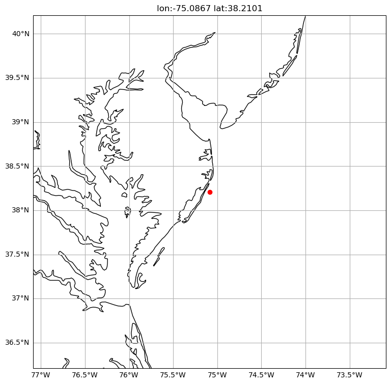
Query the various models for the appropriate data
In this cell we iterate through the various THREDDS endpoint to query for data matching the criteria specified above.
We use xarray to make our lives easier by searching for the specified location and time range.
%%time

import datetime

import matplotlib.pyplot as plt
import pandas as pd
import xarray as xr

# initialize figure
fig, ax = plt.subplots(figsize=(10, 10))

urls = {
    "gfsatlocn": "https://tds.ioos.us/thredds/dodsC/ioos/gfswave/atlocn/Best",
    "nwps": "https://tds.ioos.us/thredds/dodsC/ioos/nwps/akq/Best/LatLon_229X153-37p66N-75p76W-3",
    "gfs": "https://tds.ioos.us/thredds/dodsC/ioos/gfswave/global/Best",
}

# initialize output dataframe
df_out = pd.DataFrame({"time": []})

for key in urls.keys():

    print(f"Getting data from {urls[key]}")

    ds = xr.open_dataset(urls[key])

    data = (
        ds.filter_by_attrs(abbreviation="HTSGW")
        .sel(lat=lat, lon=lon360, method="nearest")
        .sel(time=time)
    )
    data.coords["lon"] = (data.coords["lon"] + 180) % 360 - 180
    df = data.to_dataframe().reset_index()
    df["time"] = df["time"].dt.tz_localize("UTC")

    suffix = f"_{key}"

    df_out = pd.merge_ordered(left=df, right=df_out, on="time", suffixes=[suffix, None])

    data.plot.scatter(x="time", y=list(data.data_vars)[0], ax=ax, label=key)


# add legend
ax.legend()

xmin = datetime.datetime.today() - datetime.timedelta(hours=6)
xmax = datetime.datetime.today() + datetime.timedelta(days=7)

# set limits
ax.set_xlim([xmin, xmax])

ax.set_ylabel("Significant height of wind waves [m]")

# add a line for right now
ax.vlines(datetime.datetime.today(), ymin=0, ymax=2.5, color="grey");
Getting data from https://tds.ioos.us/thredds/dodsC/ioos/gfswave/atlocn/Best
Getting data from https://tds.ioos.us/thredds/dodsC/ioos/nwps/akq/Best/LatLon_229X153-37p66N-75p76W-3
Getting data from https://tds.ioos.us/thredds/dodsC/ioos/gfswave/global/Best
CPU times: user 333 ms, sys: 56.8 ms, total: 390 ms
Wall time: 46.7 s

Next we are interested in looking at real-time data for a location near our point.
We can look at the IOOS Sensor Map to find a station and then create a timeseries plot in the tool.
Or, we can use the IOOS Sensor Map ERDDAP to search for stations in our area with appropriate data.
This searches through the ERDDAP for appropriate datasets and returns metadata about each one as a DataFrame.
import pandas as pd
from erddapy import ERDDAP

server = "https://erddap.sensors.ioos.us/erddap/"

e = ERDDAP(
    server=server,
    protocol="tabledap",
    response="csv",
)

kw = {
    "standard_name": "sea_surface_wave_significant_height",
    "min_lon": float(lon - 1),
    "max_lon": float(lon + 1),
    "min_lat": float(lat - 1),
    "max_lat": float(lat + 1),
    "min_time": "now-1day",
    "max_time": "now",
}


search_url = e.get_search_url(response="csv", **kw)

stations = pd.read_csv(search_url)

stationsLet’s get the real-time data
Now that we know what datasets match our criteria, we can go out and gather the actual values.
dataset_ids = stations["Dataset ID"]

dfs = {}


def request_station(dataset_ids):
    for dataset_id in dataset_ids:
        e.dataset_id = dataset_id

        e.variables = [
            "time",
            "longitude",
            "latitude",
            "sea_surface_wave_significant_height",
            "sea_surface_wave_mean_period",
        ]

        e.constraints = {
            "time>=": "now-2days",
            "time<": "now",
        }

        df = e.to_pandas().dropna()
        df["time (UTC)"] = pd.to_datetime(df["time (UTC)"])
        dfs[dataset_id] = df

    return dfs


dfs = request_station(dataset_ids)
Make a map of the stations we found in our search.
import cartopy.crs as ccrs
import matplotlib.pyplot as plt
from cartopy.mpl.ticker import LatitudeFormatter, LongitudeFormatter


def make_map():
    fig, ax = plt.subplots(
        figsize=(9, 9), subplot_kw=dict(projection=ccrs.PlateCarree())
    )
    ax.coastlines(resolution="10m")
    lon_formatter = LongitudeFormatter(zero_direction_label=True)
    lat_formatter = LatitudeFormatter()
    ax.xaxis.set_major_formatter(lon_formatter)
    ax.yaxis.set_major_formatter(lat_formatter)

    return fig, ax


fig, ax = make_map()
lons, lats = [], []
for station, df in dfs.items():
    lon, lat = (
        df["longitude (degrees_east)"].unique(),
        df["latitude (degrees_north)"].unique(),
    )
    lons.extend(lon)
    lats.extend(lat)
    ax.plot(lon, lat, marker="o", label=station)

dx = dy = 0.25
extent = min(lons) - dx, max(lons) + dx, min(lats) - dy, max(lats) + dy
ax.set_extent(extent)

ax.set_xticks([extent[0], extent[1]], crs=ccrs.PlateCarree())
ax.set_yticks([extent[2], extent[3]], crs=ccrs.PlateCarree())
ax.legend();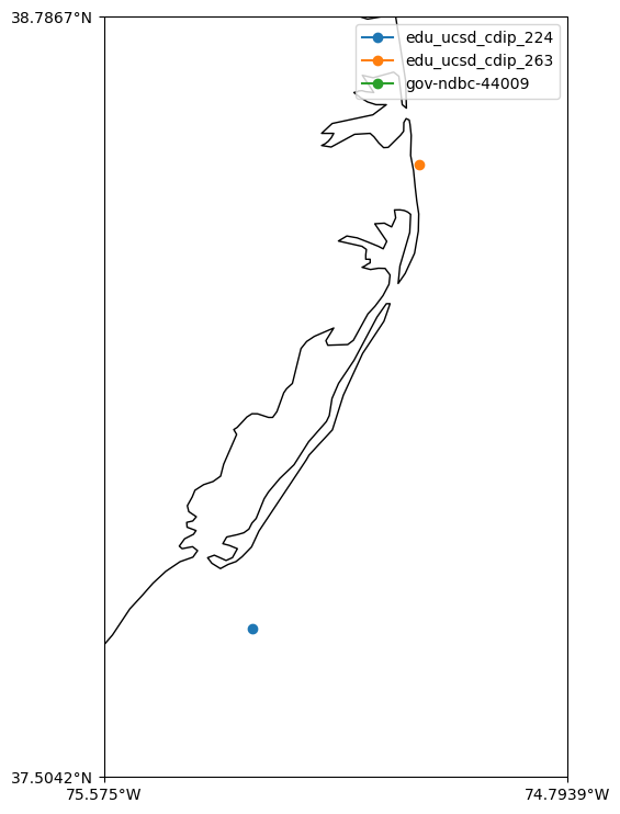
Let’s look at the last day of observations for those stations.
import datetime

import matplotlib.dates as dates
import pytz

kw = {
    "marker": "o",
    "linestyle": "none",
}


def station_scatter(df, station, ax):
    df.plot(
        ax=ax[0],
        x="time (UTC)",
        y="sea_surface_wave_significant_height (m)",
        label=station,
        **kw,
    )

    df.plot(
        ax=ax[1],
        x="time (UTC)",
        y="sea_surface_wave_mean_period (s)",
        **kw,
        legend=False,
    )


fig, ax = plt.subplots(ncols=1, nrows=2, figsize=(10, 7), sharex=True)


for station, df in dfs.items():
    station_scatter(df, station, ax)

ax[0].set_ylabel("sea_surface_wave_significant_height (m)")
ax[0].set_xlabel("time (UTC)")
ax[0].grid(True)
ax[1].set_ylabel("sea_surface_wave_mean_period (s)")
ax[1].set_xlabel("time (UTC)")
ax[1].grid(True)

plt.axvline(datetime.datetime.now(pytz.timezone("UTC")), color="green", linestyle=":");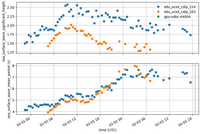
Overlay models with in-situ observations
import datetime

import pytz

dfs["gdfs"] = df_out[
    [
        "time",
        "Significant_height_of_combined_wind_waves_and_swell_surface_gfs",
        "lat_gfs",
        "lon_gfs",
    ]
].copy()

dfs["nwps"] = df_out[
    [
        "time",
        "Significant_height_of_combined_wind_waves_and_swell_surface_nwps",
        "lat_nwps",
        "lon_nwps",
    ]
].copy()

dfs["gdfs"].rename(
    columns={
        "Significant_height_of_combined_wind_waves_and_swell_surface_gfs": "sea_surface_wave_significant_height (m)",
        "time": "time (UTC)",
        "lat_gfs": "latitude (degrees_north)",
        "lon_gfs": "longitude (degrees_east)",
    },
    inplace=True,
)
dfs["nwps"].rename(
    columns={
        "Significant_height_of_combined_wind_waves_and_swell_surface_nwps": "sea_surface_wave_significant_height (m)",
        "time": "time (UTC)",
        "lat_nwps": "latitude (degrees_north)",
        "lon_nwps": "longitude (degrees_east)",
    },
    inplace=True,
)

dfs.keys()


def station_scatter(df, station, ax):
    ax.plot(
        dates.date2num(df["time (UTC)"]),
        df["sea_surface_wave_significant_height (m)"],
        label=station,
        linestyle="-",
        markersize=2,
    )


fig, ax = plt.subplots(ncols=1, nrows=1, figsize=(10, 5))
ax.set_ylabel("sea_surface_wave_significant_height (m)")
ax.set_xlabel("time (UTC)")
ax.grid(True)


for station, df in dfs.items():
    station_scatter(df, station, ax)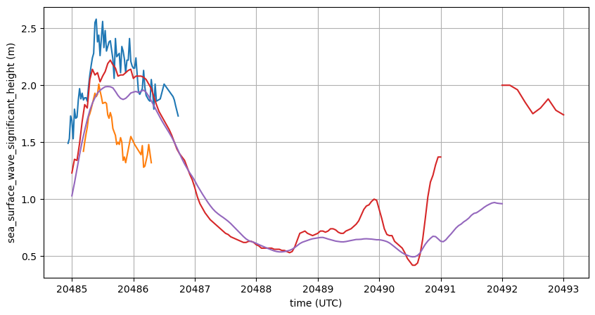
Combine the timeseries and map into one figure
from bokeh.embed import file_html
from bokeh.plotting import figure
from bokeh.resources import CDN
from folium import IFrame

# Plot defaults.
tools = "pan,box_zoom,reset"
width, height = 750, 250


def make_plot(series, station):
    p = figure(
        toolbar_location="above",
        x_axis_type="datetime",
        width=width,
        height=height,
        tools=tools,
        title=station,
    )
    line = p.line(
        x=series.index,
        y=series.values,
        line_width=5,
        line_cap="round",
        line_join="round",
    )
    return p, line


def make_marker(p, location, fname):
    html = file_html(p, CDN, fname)
    iframe = IFrame(html, width=width + 45, height=height + 80)

    popup = folium.Popup(iframe, max_width=2650)
    icon = folium.Icon(color="green", icon="stats")
    marker = folium.Marker(location=location, popup=popup, icon=icon)
    return marker
import folium
import folium.plugins
m = folium.Map()
folium.plugins.Fullscreen().add_to(m)
for station, df in dfs.items():
if not df.empty:
lon = df["longitude (degrees_east)"].dropna().unique().squeeze()
lat = df["latitude (degrees_north)"].dropna().unique().squeeze()
cols = ["time (UTC)", "sea_surface_wave_significant_height (m)"]
df = df[cols].set_index("time (UTC)").squeeze()
df.index = df.index.tz_localize(None)
p, _ = make_plot(df, station=station)
marker = make_marker(p, location=(lat, lon), fname=station)
marker.add_to(m)
m.fit_bounds(m.get_bounds())
m