Using r-obistools and r-obis to explore the OBIS database
Created: 2018-02-20
Modified: 2026-02-04
The Ocean Biogeographic Information System (OBIS) is an open-access data and information system for marine biodiversity for science, conservation and sustainable development.
In this example we will use R libraries obistools and robis to search data regarding marine turtles occurrence in the South Atlantic Ocean.
Let’s start by loading the R-to-Python extension and check the database for the 7 known species of marine turtles found in the world’s oceans.
%load_ext rpy2.ipython%%R -o matches
library(obistools)
species <- c(
'Caretta caretta',
'Chelonia mydas',
'Dermochelys coriacea',
'Eretmochelys imbricata',
'Lepidochelys kempii',
'Lepidochelys olivacea',
'Natator depressa'
)
matches = match_taxa(species, ask=FALSE)R[write to console]: 7 names, 0 without matches, 0 with multiple matches
matchesWe got a nice DataFrame back with records for all 7 species of turtles and their corresponding ID in the database.
Now let us try to obtain the occurrence data for the South Atlantic. We will need a vector geometry for the ocean basin in the well-known test (WKT) format to feed into the robis occurrence function.
In this example we converted a South Atlantic shapefile to WKT with geopandas, but one can also obtain geometries by simply drawing them on a map with iobis maptool.
from pathlib import Path

import geopandas

fname = Path("..", "data", "oceans.shp")

gdf = geopandas.read_file(fname)

sa = gdf.loc[gdf["Oceans"] == "South Atlantic Ocean"]["geometry"].loc[0]

atlantic = sa.wkt
%%R -o turtles -i atlantic
library(robis)
turtles = occurrence(
species,
geometry=atlantic,
)
names(turtles)Retrieved 5000 records of approximately 5620 (88%)
Retrieved 5620 records of approximately 5620 (100%)
  [1] "date_year"                     "scientificNameID"
  [3] "scientificName"                "dynamicProperties"
  [5] "superfamilyid"                 "individualCount"
  [7] "associatedReferences"          "dropped"
  [9] "aphiaID"                       "decimalLatitude"
 [11] "type"                          "taxonRemarks"
 [13] "phylumid"                      "familyid"
 [15] "catalogNumber"                 "occurrenceStatus"
 [17] "basisOfRecord"                 "superclass"
 [19] "modified"                      "id"
 [21] "order"                         "recordNumber"
 [23] "georeferencedDate"             "superclassid"
 [25] "verbatimEventDate"             "dataset_id"
 [27] "decimalLongitude"              "collectionCode"
 [29] "date_end"                      "speciesid"
 [31] "occurrenceID"                  "superfamily"
 [33] "suborderid"                    "license"
 [35] "date_start"                    "organismID"
 [37] "genus"                         "dateIdentified"
 [39] "ownerInstitutionCode"          "bibliographicCitation"
 [41] "eventDate"                     "scientificNameAuthorship"
 [43] "absence"                       "taxonRank"
 [45] "genusid"                       "originalScientificName"
 [47] "marine"                        "subphylumid"
 [49] "vernacularName"                "institutionCode"
 [51] "date_mid"                      "identificationRemarks"
 [53] "class"                         "suborder"
 [55] "nomenclaturalCode"             "orderid"
 [57] "datasetName"                   "geodeticDatum"
 [59] "taxonomicStatus"               "kingdom"
 [61] "waterBody"                     "specificEpithet"
 [63] "classid"                       "phylum"
 [65] "species"                       "coordinatePrecision"
 [67] "organismRemarks"               "subphylum"
 [69] "datasetID"                     "occurrenceRemarks"
 [71] "family"                        "category"
 [73] "kingdomid"                     "node_id"
 [75] "flags"                         "sss"
 [77] "shoredistance"                 "sst"
 [79] "bathymetry"                    "coordinateUncertaintyInMeters"
 [81] "eventTime"                     "sex"
 [83] "footprintWKT"                  "lifeStage"
 [85] "wrims"                         "references"
 [87] "year"                          "language"
 [89] "day"                           "locality"
 [91] "month"                         "samplingProtocol"
 [93] "eventID"                       "startDayOfYear"
 [95] "accessRights"                  "country"
 [97] "habitat"                       "municipality"
 [99] "stateProvince"                 "behavior"
[101] "recordedBy"                    "maximumDepthInMeters"
[103] "georeferenceRemarks"           "minimumElevationInMeters"
[105] "maximumElevationInMeters"      "minimumDepthInMeters"
[107] "depth"                         "continent"
[109] "fieldNotes"                    "rightsHolder"
[111] "associatedMedia"               "taxonConceptID"
[113] "organismQuantity"              "organismQuantityType"
[115] "fieldNumber"                   "eventRemarks"
[117] "preparations"                  "identifiedBy"
[119] "typeStatus"                    "otherCatalogNumbers"
[121] "locationID"
set(turtles["scientificName"]){'Caretta caretta',
'Chelonia mydas',
'Dermochelys coriacea',
'Eretmochelys imbricata',
'Lepidochelys kempii',
'Lepidochelys olivacea'}Note that there are no occurrences for Natator depressa (Flatback sea turtle) in the South Atlantic. The Flatback sea turtle can only be found in the waters around the Australian continental shelf.
With ggplot2 we can quickly put together a of occurrences over time.
%%R

turtles$year <- as.numeric(format(as.Date(turtles$eventDate), "%Y"))
table(turtles$year)

library(ggplot2)

ggplot() +
 geom_histogram(
     data=turtles,
     aes(x=year, fill=scientificName),
     binwidth=5) +
 scale_fill_brewer(palette='Paired')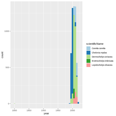
One would guess that the 2010 count increase would be due to an increase in the sampling effort, but the drop around 2010 seems troublesome. It can be a real threat to these species, or the observation efforts were defunded.
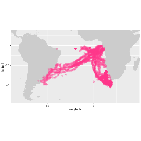
To explore this dataset further we can make use of the obistools’ R package. obistools has many visualization and quality control routines built-in. Here is an example on how to use plot_map to quickly visualize the data on a geographic context.
%%R

library(dplyr)

coriacea <- turtles %>% filter(species=='Dermochelys coriacea')
plot_map(coriacea, zoom=TRUE)
R[write to console]:
Attaching package: ‘dplyr’
R[write to console]: The following objects are masked from ‘package:stats’:
filter, lag
R[write to console]: The following objects are masked from ‘package:base’:
intersect, setdiff, setequal, union
However, if we want to create a slightly more elaborate map with clusters and informative pop-ups, can use the python library folium.instead.
import folium
from pandas import DataFrame


def filter_df(df):
    return df[["institutionCode", "individualCount", "sex", "eventDate"]]


def make_popup(row):
    classes = "table table-striped table-hover table-condensed table-responsive"
    html = DataFrame(row).to_html(classes=classes)
    return folium.Popup(html)


def make_marker(row, popup=None):
    location = row["decimalLatitude"], row["decimalLongitude"]
    return folium.Marker(location=location, popup=popup)
from folium.plugins import MarkerCluster
species_found = sorted(set(turtles["scientificName"]))
clusters = {s: MarkerCluster() for s in species_found}
groups = {s: folium.FeatureGroup(name=s) for s in species_found}turtlesm = folium.Map()
for turtle in species_found:
df = turtles.loc[turtles["scientificName"] == turtle]
for k, row in df.iterrows():
popup = make_popup(filter_df(row))
make_marker(row, popup=popup).add_to(clusters[turtle])
clusters[turtle].add_to(groups[turtle])
groups[turtle].add_to(m)
m.fit_bounds(m.get_bounds())
folium.LayerControl().add_to(m)
mWe can get fancy and use shapely to “merge” the points that are on the ocean and get an idea of migrations routes.
%%R -o land

land <- check_onland(turtles)

plot_map(land, zoom=TRUE)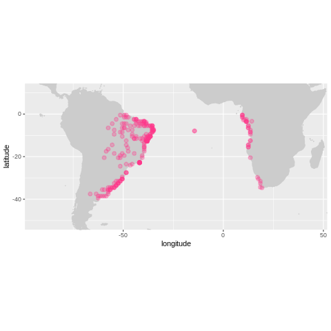
First let’s remove the entries that are on land.
turtles.set_index("id", inplace=True)
land.set_index("id", inplace=True)
mask = turtles.index.isin(land.index)
ocean = turtles[~mask]
Now we can use shapely’s buffer to “connect” the points that are close to each other to visualize a possible migration path.
from palettable.cartocolors.qualitative import Bold_6
from shapely.geometry import MultiPoint

colors = {s: c for s, c in zip(species_found, Bold_6.hex_colors)}
style_function = lambda color: (
    lambda feature: dict(color=color, weight=2, opacity=0.6)
)

m = folium.Map()

for turtle in species_found:
    df = ocean.loc[ocean["scientificName"] == turtle]
    positions = MultiPoint(
        list(zip(df["decimalLongitude"].values, df["decimalLatitude"].values))
    ).buffer(distance=2)
    folium.GeoJson(
        positions.__geo_interface__,
        name=turtle,
        tooltip=turtle,
        style_function=style_function(color=colors[turtle]),
    ).add_to(m)

m.fit_bounds(m.get_bounds())
folium.LayerControl().add_to(m)

mOne interesting feature of this map is Dermochelys coriacea’s migration between Brazilian and African shores.
More information on Dermochelys coriacea and the other Sea Turtles can be found in the species IUCN red list.