import logging
import subprocess
import sys

COLAB = "google.colab" in sys.modules


def _install(package):
    if COLAB:
        ans = input(f"Install { package }? [y/n]:")
        if ans.lower() in ["y", "yes"]:
            subprocess.check_call(
                [sys.executable, "-m", "pip", "install", "--quiet", package]
            )
            print(f"{ package } installed!")


def _colab_install_missing_deps(deps):
    import importlib

    for dep in deps:
        if importlib.util.find_spec(dep) is None:
            if dep == "iris":
                dep = "scitools-iris"
            _install(dep)


deps = ["geoplot", "pyobis"]
_colab_install_missing_deps(deps)


logging.disable(sys.maxsize)

Using pyobis to query for known datasets¶

Created: 2022-11-23

Updated: 2026-05-04

Author: Mathew Biddle

This notebook uses the pyobis Python package to query the OBIS API for datasets associated with projects funded under the United States Marine Biodiversity Observation Network. The notebook walks through the process for querying the OBIS api for a specific institution, then using the resultant datasets to gather the locations of all the occurrences using the pyobis package.

The US Marine Biodiversity Observation Network (US MBON) is an interagency initiative that seeks to coordinate across sectors and government to characterize biodiversity and understand drivers of change. US MBON represents a broad, collaborative effort to address the need for systematic collection and sharing of marine life information, ensure that information is available for decision-making and management from local to national levels, and document marine biodiversity status and trends in the face of human- and climate-induced change using a range of technologies and approaches. Through the National Oceanographic Partnership Program, NOAA, NASA, Office of Naval Research, and BOEM have invested in US MBON since 2014, most recently announcing new five year projects in 2022.

import pyobis

pyobis.__version__

'1.6.1'

First off, let’s look through the available institutions at OBIS and find the US MBON one.

Hint: We know the name of the institution is United States Marine Biodiversity Observation Network.

import pandas as pd

pd.set_option("max_colwidth", 400)

url = "https://api.obis.org/v3/institute"

institutes = pd.read_json(url)

df_inst = pd.DataFrame.from_records(institutes["results"])

df_inst.dropna(inplace=True)

df_inst["id"] = df_inst["id"].astype(int)

institution = df_inst.loc[
    df_inst["name"].str.contains(
        "United States Marine Biodiversity Observation", na=False
    )
]

institution

Well that looks like the institution we’re after!

Using the id we can check it out on the OBIS website: https://obis.org/organization/23070

Yes, that does look like what we want. Now let’s use that id to query OBIS for all associated datasets.

institution_id = institution["id"].tolist()[0]

institution_id

23070

Collect metadata about all of the datasets¶

Here we use the institution_id collected from OBIS to query the API for metadata on the datasets associated with that id.

First, we build the API call, then we bring it into a Pandas DataFrame and create additional fields for use later.

import pyobis

query = pyobis.dataset.search(instituteid=institution_id)

df = pd.DataFrame(query.execute())

df_meta = pd.DataFrame.from_records(df["results"])

# create a column for the human readable short name of the datasets
df_meta["short_name"] = df_meta["url"].str.split("=", expand=True)[1]

# create another column to group datasets by, which removes the year from the short names
df_meta["short_name_group"] = df_meta["short_name"].replace(r"\d", "", regex=True)

df_meta.head(5)

df_meta[["short_name", "short_name_group"]].describe()

Read to geopandas and plot the bounding boxes¶

Next we want to make a simple map of the coverage each dataset has. We can use the extent field directly in geopandas to make a simple map.

from datetime import datetime

import cartopy.io.shapereader as shpreader
import geopandas
import matplotlib.pyplot as plt

gdf = geopandas.GeoDataFrame(
    df_meta, geometry=geopandas.GeoSeries.from_wkt(df_meta["extent"])
)
gdf.set_crs("epsg:4326", inplace=True)

fig, ax = plt.subplots(
    figsize=(20, 15),
)

gdf.plot(
    ax=ax,
    zorder=10,
    alpha=0.5,
    column="short_name_group",
    legend=True,
    cmap="turbo",
)

leg = ax.get_legend()

leg.set_bbox_to_anchor((0.0, 0.0, 1.2, 0.9))

shpfilename = shpreader.natural_earth(
    resolution="110m",
    category="cultural",
    name="admin_0_countries",
)
world = geopandas.read_file(shpfilename)
world = world.to_crs(gdf.crs)

# bound map to US.
world.loc[world["ISO_A3"] == "USA"].plot(
    ax=ax, color="lightgrey", edgecolor="black", zorder=1
)

today = datetime.now().strftime("%Y-%m-%d")

ax.set_title(
    f"Sampling coverage map\nTotal dataset records contributed to OBIS from the US MBON network as of {today}: {gdf.records.sum() }"
)

ax.set_axis_off();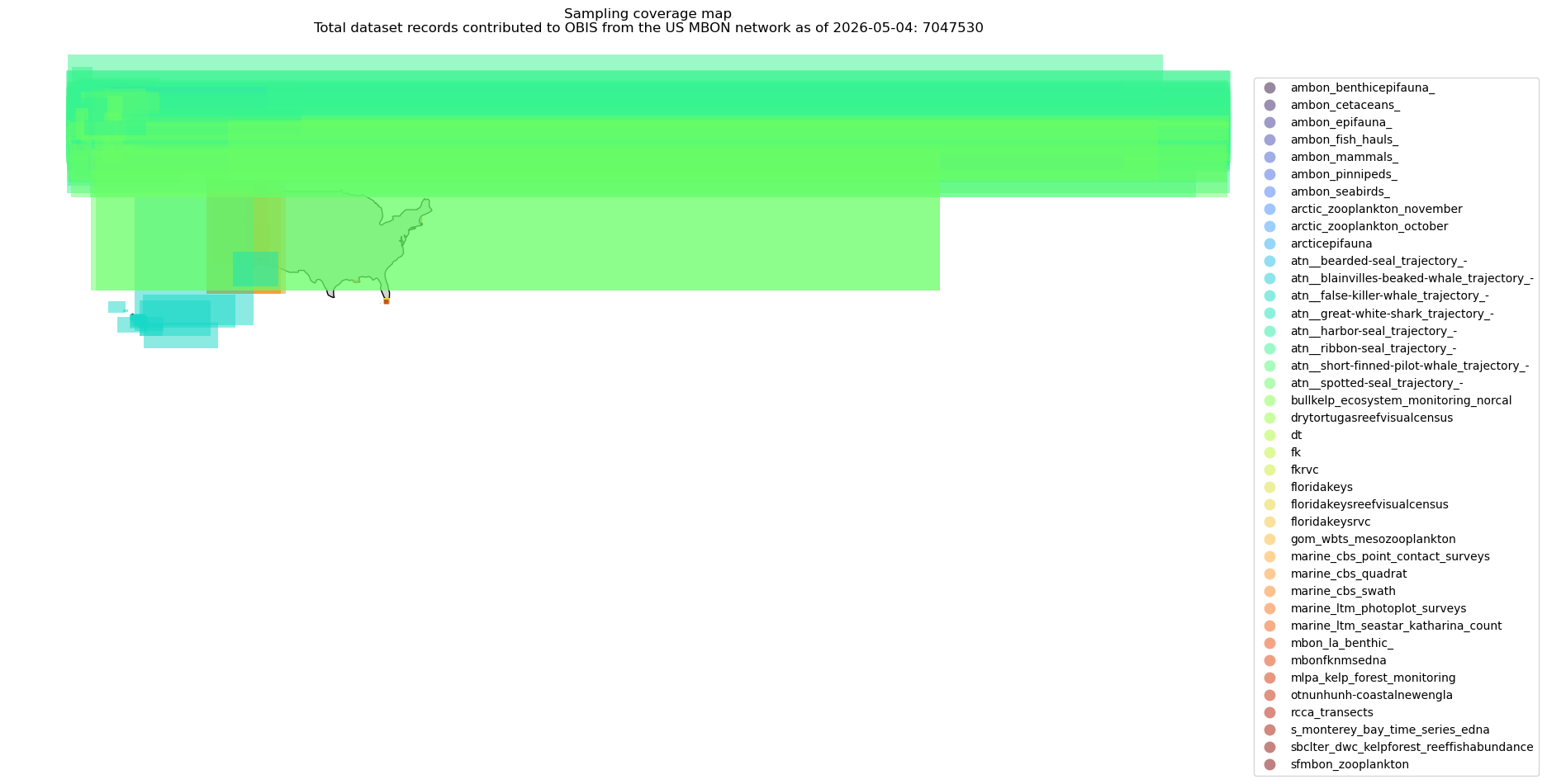

gdf.explore(column="short_name")

Save as a geojson¶

Since we have the data, why don’t we write this out to a geoJson file to interact with on GitHub.

fname = f"US_MBON_bounding_boxes_{today.replace('-','')}.geojson"

# can"t export fields with lists or dictionaries - breaks the format.
gdf[["id", "title", "url", "geometry"]].to_file(fname, driver="GeoJSON")

Query the OBIS aggregated points¶

Now that we know the general area for where our observations are made, let’s dig a little deeper into each dataset.

We can use pyobis.occurrences.getpoints() to return all of the points for each dataset, aggregated to Geohash precision 8.

If we’d like a little more metadata about each of the aggregated points, we can query by dataset to collect the aggregated points and some useful metadata.

combined = pd.DataFrame()

query = pyobis.dataset.search(instituteid=institution_id)
df = pd.DataFrame(query.execute())
df_meta = pd.DataFrame.from_records(df["results"])


for datasetid in df_meta["id"]:
    dset = pyobis.occurrences.getpoints(datasetid=datasetid).execute()

    meta = pyobis.dataset.get(id=datasetid).execute()["results"][0]
    short_name = meta["url"].split("=")[-1]

    df = pd.DataFrame(dset)

    df["dataset_id"] = datasetid
    df["short_name"] = meta["url"].split("=")[-1]
    df["short_name_group"] = df["short_name"].replace(r"\d", "", regex=True)
    df["url"] = meta["url"]
    df["metadata"] = str(meta)

    df[["decimalLongitude", "decimalLatitude"]] = pd.DataFrame(
        df["coordinates"].tolist()
    )

    combined = pd.concat([combined, df], ignore_index=True)


gdf_ghsh = geopandas.GeoDataFrame(
    combined[
        ["dataset_id", "url", "short_name_group", "decimalLatitude", "decimalLongitude"]
    ],
    geometry=geopandas.points_from_xy(
        combined.decimalLongitude, combined.decimalLatitude
    ),
    crs="epsg:4326",
)


fig, ax = plt.subplots(figsize=(20, 15))


gdf_ghsh.plot(
    ax=ax,
    zorder=10,
    alpha=0.5,
    column="short_name_group",
    legend=True,
)

world.loc[world["ISO_A3"] == "USA"].plot(
    ax=ax, color="lightgrey", edgecolor="white", zorder=1
)

now = datetime.now()

today = now.strftime("%Y-%m-%d")

ax.set_title(
    f"Total aggregated occurrence records contributed to OBIS from the US MBON network as of {today}: {gdf_ghsh.shape[0]}"
)

ax.set_axis_off();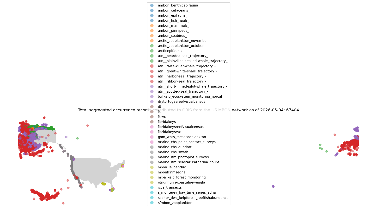

Let’s explore those points a little more with geopandas.GeoDataFrame.explore().

This allows you to create an interactive map based on folium/leaflet.jsInteractive map based on GeoPandas and folium/leaflet.js

gdf_ghsh.explore(column="short_name_group")

Use pyobis to return all occurrences.¶

If you are really interested in all of the records, the code below exemplifies how one might use pyobis to iterate through each dataset and collect only the coordinates to create a map.

Note: This takes a while to run!

First, let’s get all the occurrences as one huge DataFrame.

from pathlib import Path

fname = "combined_high_res.zip"
if Path(fname).exists():
    print(
        f"Loading cached {fname}. Remove this file if you want to fetch all the points again."
    )
    combined_high_res = pd.read_csv(fname, compression="zip")
else:
    combined_high_res = pd.DataFrame()
    query = pyobis.dataset.search(instituteid=institution_id)

    df = pd.DataFrame(query.execute())
    df_meta = pd.DataFrame.from_records(df["results"])

    fields = ["decimalLatitude", "decimalLongitude", "id"]

    for datasetid in df_meta["id"]:
        query = pyobis.occurrences.search(datasetid=datasetid, fields=fields)
        dset = query.execute()

        df = pd.DataFrame(dset)

        combined_high_res = pd.concat([combined_high_res, df], ignore_index=True)

    combined_high_res[["decimalLongitude", "decimalLatitude"]].to_csv(
        fname, index=False, compression="zip"
    )

Loading cached combined_high_res.zip. Remove this file if you want to fetch all the points again.

Next, let’s convert that DataFrame to a GeoDataFrame and plot the points on a map.

gdf_high_res = geopandas.GeoDataFrame(
    combined_high_res[["decimalLatitude", "decimalLongitude"]],
    geometry=geopandas.points_from_xy(
        combined_high_res.decimalLongitude, combined_high_res.decimalLatitude
    ),
    crs="epsg:4326",
)

fig, ax = plt.subplots(figsize=(20, 15))

gdf_high_res.plot.scatter(
    x="decimalLongitude",
    y="decimalLatitude",
    ax=ax,
    s=5,
    zorder=10,
    rasterized=True,
)


world.loc[world["ISO_A3"] == "USA"].plot(
    ax=ax, color="lightgrey", edgecolor="white", zorder=1
)

now = datetime.now()

today = now.strftime("%Y-%m-%d")

ax.set_title(
    f"Total occurrence records contributed to OBIS from the US MBON network as of {today}: {gdf_high_res.shape[0]}"
)

ax.set_axis_off();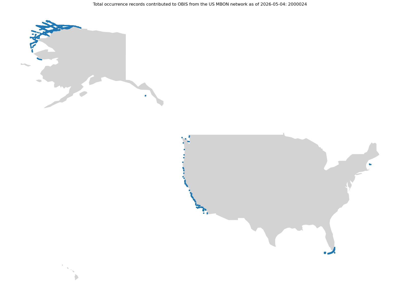

Let’s make some histograms of occurrence record distributions across latitude and longitude¶

First, we need to create the bins by which we will calculate the number of occurrences. For this example we will use 1 degree bins.

bins_lat = [i for i in range(-90, 90, 1)]
bins_lon = [i for i in range(-180, 180, 1)]

fig, ax = plt.subplots(nrows=1, ncols=2, figsize=(16, 8))

gdf_high_res.hist(
    column="decimalLatitude", bins=bins_lat, orientation="horizontal", ax=ax[0]
)

gdf_high_res.hist(
    column="decimalLongitude", bins=bins_lon, orientation="vertical", ax=ax[1]
)

array([<Axes: title={'center': 'decimalLongitude'}>], dtype=object)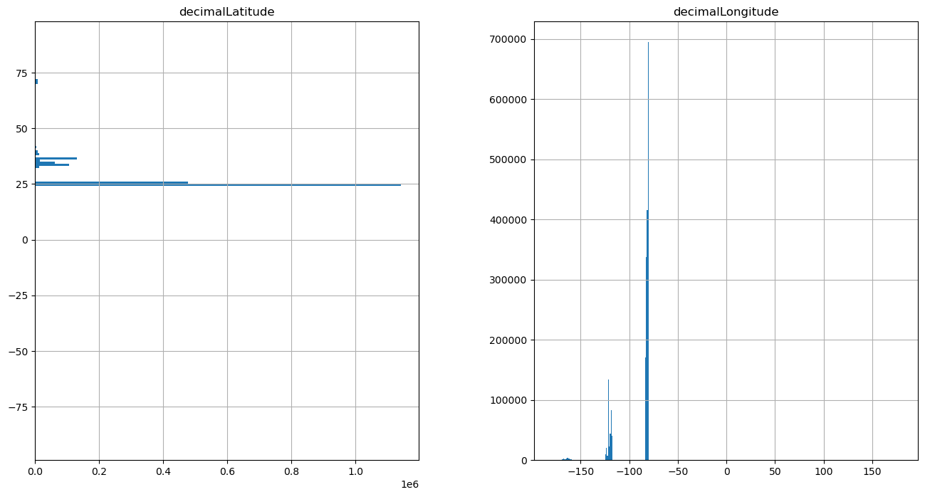

Create a grid of observations¶

1 degree x 1 degree

import numpy as np
import shapely

# total area for the grid
xmin, ymin, xmax, ymax = [-180.0, -90.0, 180.0, 90]

# how many cells across and down
n_cells = 360

# calculate the size of the cells
cell_size = (xmax - xmin) / n_cells

# create an evenly distributed GeoDataFrame for the grid described above
grid_cells = []
for x0 in np.arange(xmin, xmax + cell_size, cell_size):
    for y0 in np.arange(ymin, ymax + cell_size, cell_size):
        # bounds
        x1 = x0 - cell_size
        y1 = y0 + cell_size
        grid_cells.append(shapely.geometry.box(x0, y0, x1, y1))

cell = geopandas.GeoDataFrame(grid_cells, columns=["geometry"], crs="EPSG:4326")

# spatial join the OBIS data with the one-degree cells for where OBIS data are within cells.
merged = geopandas.sjoin(gdf_high_res, cell, how="left", predicate="within")

# make a simple count variable that we can sum for each cell
merged["n_occur"] = 1

# Compute stats per grid cell -- aggregate occurences to grid cells with dissolve
dissolve = merged.dissolve(by="index_right", aggfunc="count")

# put this into cell
cell.loc[dissolve.index, "n_occur"] = dissolve.n_occur.values

# calculate occurrence density in km^2 for each cell.
cell["area (km2)"] = cell.to_crs(epsg=3763).area / (1000**2)

cell.plot(column="n_occur", legend=True);

/home/filipe/micromamba/envs/IOOS/lib/python3.14/site-packages/shapely/measurement.py:50: RuntimeWarning: invalid value encountered in area
  return lib.area(geometry, **kwargs)

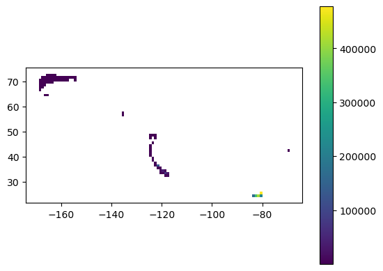
Next, let’s check out the distribution of the values for n_occur so we can make an appropriatly legible map of the distribution.

cell.describe()

/home/filipe/micromamba/envs/IOOS/lib/python3.14/site-packages/pandas/core/nanops.py:1027: RuntimeWarning: invalid value encountered in subtract
  sqr = _ensure_numeric((avg - values) ** 2)

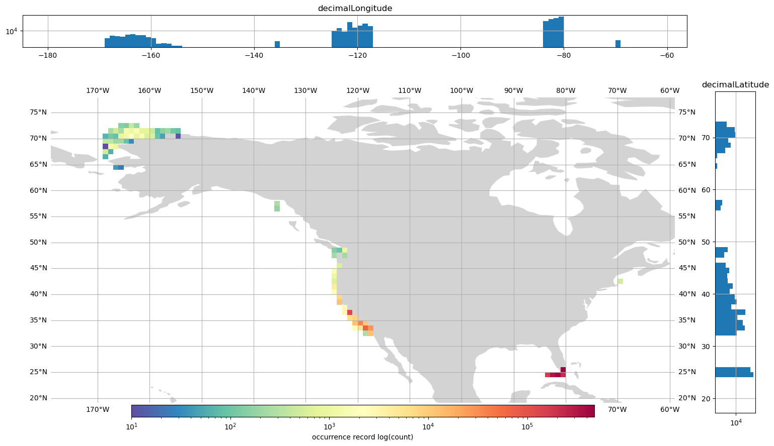
Since the distribution of n_occur covers a wide range, we will present the concentration and histogram figures as log normal distributions.

So, let’s combine the latitude and longitude histograms with the map to recreate this figure https://bbest.github.io/obis-lat-time-fig.

import geoplot
import geoplot.crs as gcrs
import matplotlib as mpl
import matplotlib.pyplot as plt
import matplotlib.ticker as mticker

norm = mpl.colors.LogNorm(vmin=cell["n_occur"].min(), vmax=cell["n_occur"].max())

projection = gcrs.PlateCarree(central_longitude=-105)

world = world.dissolve()

fig, ax = plt.subplots(
    figsize=(16, 8), facecolor="white", subplot_kw={"projection": projection}
)

geoplot.polyplot(
    world,
    facecolor="lightgray",
    edgecolor=None,
    projection=projection,
    ax=ax,
)


cax = fig.add_axes([0.225, 0.08, 0.575, 0.03])


cell = cell[~cell["n_occur"].isna()]

geoplot.choropleth(
    cell,
    hue="n_occur",
    edgecolor=None,
    projection=projection,
    ax=ax,
    cmap="Spectral_r",
    legend=True,
    legend_kwargs={
        "orientation": "horizontal",
        "cax": cax,
        "label": "occurrence record log(count)",
    },
    norm=norm,
)

gl = ax.gridlines(draw_labels=True)
gl.ylocator = mticker.FixedLocator(range(0, 90, 5))
gl.xlocator = mticker.FixedLocator(range(-170, -40, 10))


# Add histogram for distribution
ax2 = fig.add_axes([0.95, 0.090, 0.05, 0.8])

bins_lat = [i for i in range(20, 77, 1)]

gdf_high_res.hist(
    column="decimalLatitude", bins=bins_lat, orientation="horizontal", ax=ax2, log=True
)

ax3 = fig.add_axes([0.09, 1, 0.825, 0.08])

bins_lon = [i for i in range(-179, -61, 1)]

gdf_high_res.hist(
    column="decimalLongitude", bins=bins_lon, orientation="vertical", ax=ax3, log=True
);